R is the most popular language used for Statistical Computing and Data Analysis with the support of over 10, 000+ free packages in CRAN repository. Like any other programming language, R has a specific syntax which is important to understand if you want to make use of its powerful features. This article assumes R is already installed on your machine. We will be using RStudio but we can also use R command prompt by typing the following command in the command line.
$ R
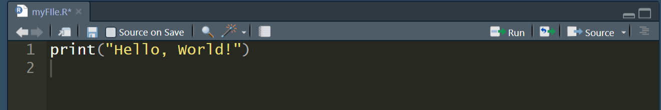
This will launch the interpreter and now let’s write a basic Hello World program to get started. 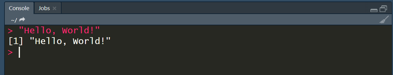 We can see that “Hello, World!” is being printed on the console. Now we can do the same thing using print() which prints to the console. Usually, we will write our code inside scripts which are called RScripts in R. To create one, write the below given code in a file and save it as myFile.R and then run it in console by writing:
Rscript myFile.R
 Output:
[1] "Hello, World!"
Syntax of R program
A program in R is made up of three things: Variables, Comments, and Keywords. Variables are used to store the data, Comments are used to improve code readability, and Keywords are reserved words that hold a specific meaning to the compiler.
Variables in R
Previously, we wrote all our code in a print() but we don’t have a way to address them as to perform further operations. This problem can be solved by using variables which like any other programming language are the name given to reserved memory locations that can store any type of data. In R, the assignment can be denoted in three ways:
- = (Simple Assignment)
- <- (Leftward Assignment)
- -> (Rightward Assignment)
Example: 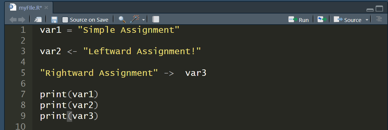 Output:
"Simple Assignment"
"Leftward Assignment!"
"Rightward Assignment"
The rightward assignment is less common and can be confusing for some programmers, so it is generally recommended to use the <- or = operator for assigning values in R.
Comments in R
Comments are a way to improve your code’s readability and are only meant for the user so the interpreter ignores it. Only single-line comments are available in R but we can also use multiline comments by using a simple trick which is shown below. Single line comments can be written by using # at the beginning of the statement. Example: 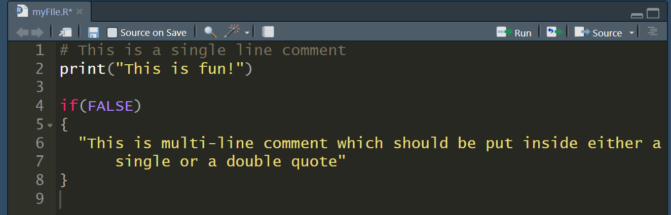 Output:
[1] "This is fun!"
From the above output, we can see that both comments were ignored by the interpreter.
Keywords in R
Keywords are the words reserved by a program because they have a special meaning thus a keyword can’t be used as a variable name, function name, etc. We can view these keywords by using either help(reserved) or ?reserved. 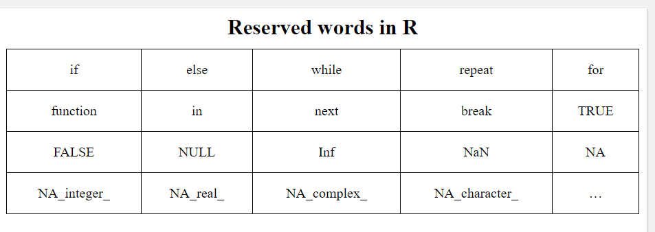
- if, else, repeat, while, function, for, in, next and break are used for control-flow statements and declaring user-defined functions.
- The ones left are used as constants like TRUE/FALSE are used as boolean constants.
- NaN defines Not a Number value and NULL are used to define an Undefined value.
- Inf is used for Infinity values.
Comments in R
Comments are generic English sentences, mostly written in a program to explain what it does or what a piece of code is supposed to do. More specifically, information that programmer should be concerned with and it has nothing to do with the logic of the code. They are completely ignored by the compiler and are thus never reflected on to the input.
The question arises here that how will the compiler know whether the given statement is a comment or not?
The answer is pretty simple. All languages use a symbol to denote a comment and this symbol when encountered by the compiler helps it to differentiate between a comment and statement.
Comments are generally used for the following purposes:
- Code Readability
- Explanation of the code or Metadata of the project
- Prevent execution of code
- To include resources
Types of Comments
There are generally three types of comments supported by languages, namely-
- Single-line Comments- Comment that only needs one line
- Multi-line Comments- Comment that requires more than one line.
- Documentation Comments- Comments that are drafted usually for a quick documentation look-up
Note: R doesn’t support Multi-line and Documentation comments. It only supports single-line comments drafted by a ‘#’ symbol.
Comments in R
As stated in the Note provided above, currently R doesn’t have support for Multi-line comments and documentation comments. R provides its users with single-lined comments in order to add information about the code.
Single-Line Comments in R
Single-line comments are comments that require only one line. They are usually drafted to explain what a single line of code does or what it is supposed to produce so that it can help someone referring to the source code.
Just like python single-line comments, any statement starting with “#” is a comment in R.
Syntax:
# comment statement
Example 1:
# geeksforgeeks |
The above code when executed will not produce any output, because R will consider the statement as a comment and hence the compiler will ignore the line.
Example 2:
# R program to add two numbers # Assigning values to variablesa <-9b <-4 # Printing sumprint(a +b) |
Output:
[1] 13
Commenting Multiple Lines
As stated earlier that R doesn’t support multi-lined comments, but to make the commenting process easier, R allows commenting multiple single lines at once. There are two ways to add multiple single-line comments in R Studio:
- First way: Select the multiple lines which you want to comment using the cursor and then use the key combination “control + shift + C” to comment or uncomment the selected lines.
- Second way: The other way is to use the GUI, select the lines which you want to comment by using the cursor and click on “Code” in menu, a pop-up window pops out in which we need to select “Comment/Uncomment Lines” which appropriately comments or uncomment the lines which you have selected.
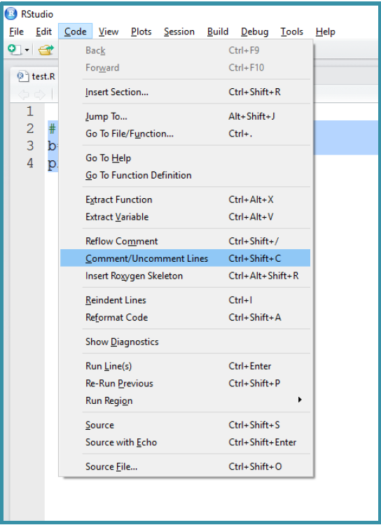
This makes the process of commenting a block of code easier and faster than adding # before each line one at a time.
R Operators
Operators are the symbols directing the compiler to perform various kinds of operations between the operands. Operators simulate the various mathematical, logical, and decision operations performed on a set of Complex Numbers, Integers, and Numericals as input operands.
R Operators
R supports majorly four kinds of binary operators between a set of operands. In this article, we will see various types of operators in R Programming language and their usage.
Types of the operator in R language
- Arithmetic Operators
- Logical Operators
- Relational Operators
- Assignment Operators
- Miscellaneous Operator
Arithmetic Operators
Arithmetic operations in R simulate various math operations, like addition, subtraction, multiplication, division, and modulo using the specified operator between operands, which may be either scalar values, complex numbers, or vectors. The R operators are performed element-wise at the corresponding positions of the vectors.
Addition operator (+)
The values at the corresponding positions of both operands are added. Consider the following R operator snippet to add two vectors:
- R
a <- c (1, 0.1)b <- c (2.33, 4)print (a+b) |
Output : 3.33 4.10
Subtraction Operator (-)
The second operand values are subtracted from the first. Consider the following R operator snippet to subtract two variables:
- R
a <- 6b <- 8.4print (a-b) |
Output : -2.4
Multiplication Operator (*)
The multiplication of corresponding elements of vectors and Integers are multiplied with the use of the ‘*’ operator.
- R
|
Output : 20 20
Division Operator (/)
The first operand is divided by the second operand with the use of the ‘/’ operator.
- R
a <- 10b <- 5print (a/b) |
Output : 2
Power Operator (^)
The first operand is raised to the power of the second operand.
- R
a <- 4b <- 5print(a^b) |
Output : 1024
Modulo Operator (%%)
The remainder of the first operand divided by the second operand is returned.
- R
list1<- c(2, 22)list2<-c(2,4)print(list1 %% list2) |
Output : 0 2
The following R code illustrates the usage of all Arithmetic R operators.
- R
# R program to illustrate# the use of Arithmetic operatorsvec1 <- c(0, 2)vec2 <- c(2, 3)# Performing operations on Operandscat ("Addition of vectors :", vec1 + vec2, "\n")cat ("Subtraction of vectors :", vec1 - vec2, "\n")cat ("Multiplication of vectors :", vec1 * vec2, "\n")cat ("Division of vectors :", vec1 / vec2, "\n")cat ("Modulo of vectors :", vec1 %% vec2, "\n")cat ("Power operator :", vec1 ^ vec2) |
Output
Addition of vectors : 2 5
Subtraction of vectors : -2 -1
Multiplication of vectors : 0 6
Division of vectors : 0 0.6666667
Modulo of vectors : 0 2
Power operator : 0 8
Logical Operators
Logical operations in R simulate element-wise decision operations, based on the specified operator between the operands, which are then evaluated to either a True or False boolean value. Any non-zero integer value is considered as a TRUE value, be it a complex or real number.
Element-wise Logical AND operator (&)
Returns True if both the operands are True.
- R
list1 <- c(TRUE, 0.1)list2 <- c(0,4+3i)print(list1 & list2) |
Output : FALSE   TRUE
Any non zero integer value is considered as a TRUE value, be it complex or real number.
Element-wise Logical OR operator (|)
Returns True if either of the operands is True.
- R
list1 <- c(TRUE, 0.1)list2 <- c(0,4+3i)print(list1|list2) |
Output : TRUE TRUE
NOT operator (!)
A unary operator that negates the status of the elements of the operand.
- R
list1 <- c(0,FALSE)print(!list1) |
Output : TRUE TRUE
Logical AND operator (&&)
Returns True if both the first elements of the operands are True.
- R
list1 <- c(TRUE, 0.1)list2 <- c(0,4+3i)print(list1 && list2) |
Output : FALSE
Compares just the first elements of both the lists.
Logical OR operator (||)
Returns True if either of the first elements of the operands is True.
- R
list1 <- c(TRUE, 0.1)list2 <- c(0,4+3i)print(list1||list2) |
Output : TRUE
The following R code illustrates the usage of all Logical Operators in R:
- R
# R program to illustrate# the use of Logical operatorsvec1 <- c(0,2)vec2 <- c(TRUE,FALSE)# Performing operations on Operandscat ("Element wise AND :", vec1 & vec2, "\n")cat ("Element wise OR :", vec1 | vec2, "\n")cat ("Logical AND :", vec1 && vec2, "\n")cat ("Logical OR :", vec1 || vec2, "\n")cat ("Negation :", !vec1) |
Output
Element wise AND : FALSE FALSE
Element wise OR : TRUE TRUE
Logical AND : FALSE
Logical OR : TRUE
Negation : TRUE FALSE
Relational Operators
The relational operators in R carry out comparison operations between the corresponding elements of the operands. Returns a boolean TRUE value if the first operand satisfies the relation compared to the second. A TRUE value is always considered to be greater than the FALSE.
Less than (<)
Returns TRUE if the corresponding element of the first operand is less than that of the second operand. Else returns FALSE.
- R
list1 <- c(TRUE, 0.1,"apple")list2 <- c(0,0.1,"bat")print(list1<list2) |
Output : FALSE FALSE TRUE
Less than equal to (<=)
Returns TRUE if the corresponding element of the first operand is less than or equal to that of the second operand. Else returns FALSE.
- R
list1 <- c(TRUE, 0.1, "apple")list2 <- c(TRUE, 0.1, "bat")# Convert lists to character stringslist1_char <- as.character(list1)list2_char <- as.character(list2)# Compare character stringsprint(list1_char <= list2_char) |
Output : TRUE TRUE TRUE
Greater than (>)
Returns TRUE if the corresponding element of the first operand is greater than that of the second operand. Else returns FALSE.
- R
list1 <- c(TRUE, 0.1, "apple")list2 <- c(TRUE, 0.1, "bat")print(list1_char > list2_char) |
Output : FALSE FALSE FALSE
Greater than equal to (>=)
Returns TRUE if the corresponding element of the first operand is greater or equal to that of the second operand. Else returns FALSE.
- R
list1 <- c(TRUE, 0.1, "apple")list2 <- c(TRUE, 0.1, "bat")print(list1_char >= list2_char) |
Output : TRUE TRUE FALSE
Not equal to (!=)
Returns TRUE if the corresponding element of the first operand is not equal to the second operand. Else returns FALSE.
- R
list1 <- c(TRUE, 0.1,'apple')list2 <- c(0,0.1,"bat")print(list1!=list2) |
Output : TRUE FALSE TRUE
The following R code illustrates the usage of all Relational Operators in R:
- R
# R program to illustrate# the use of Relational operatorsvec1 <- c(0, 2)vec2 <- c(2, 3)# Performing operations on Operandscat ("Vector1 less than Vector2 :", vec1 < vec2, "\n")cat ("Vector1 less than equal to Vector2 :", vec1 <= vec2, "\n")cat ("Vector1 greater than Vector2 :", vec1 > vec2, "\n")cat ("Vector1 greater than equal to Vector2 :", vec1 >= vec2, "\n")cat ("Vector1 not equal to Vector2 :", vec1 != vec2, "\n") |
Output
Vector1 less than Vector2 : TRUE TRUE
Vector1 less than equal to Vector2 : TRUE TRUE
Vector1 greater than Vector2 : FALSE FALSE
Vector1 greater than equal to Vector2 : FALSE FALSE
Vector1 not equal to Vector2 : TRUE TRUE
Assignment Operators
Assignment operators in R are used to assigning values to various data objects in R. The objects may be integers, vectors, or functions. These values are then stored by the assigned variable names. There are two kinds of assignment operators: Left and Right
Left Assignment (<- or <<- or =)
Assigns a value to a vector.
- R
vec1 = c("ab", TRUE)print (vec1) |
Output : "ab" "TRUE"
Right Assignment (-> or ->>)
Assigns value to a vector.
- R
c("ab", TRUE) ->> vec1print (vec1) |
Output : "ab" "TRUE"
The following R code illustrates the usage of all Relational Operators in R:
- R
# R program to illustrate# the use of Assignment operatorsvec1 <- c(2:5)c(2:5) ->> vec2vec3 <<- c(2:5)vec4 = c(2:5)c(2:5) -> vec5# Performing operations on Operandscat ("vector 1 :", vec1, "\n")cat("vector 2 :", vec2, "\n")cat ("vector 3 :", vec3, "\n")cat("vector 4 :", vec4, "\n")cat("vector 5 :", vec5) |
Output
vector 1 : 2 3 4 5
vector 2 : 2 3 4 5
vector 3 : 2 3 4 5
vector 4 : 2 3 4 5
vector 5 : 2 3 4 5
Miscellaneous Operators
These are the mixed operators in R that simulate the printing of sequences and assignment of vectors, either left or right-handed.
%in% Operator
Checks if an element belongs to a list and returns a boolean value TRUE if the value is present else FALSE.
- R
val <- 0.1list1 <- c(TRUE, 0.1,"apple")print (val %in% list1) |
Output : TRUE
Checks for the value 0.1 in the specified list. It exists, therefore, prints TRUE.
%*% Operator
This operator is used to multiply a matrix with its transpose. Transpose of the matrix is obtained by interchanging the rows to columns and columns to rows. The number of columns of the first matrix must be equal to the number of rows of the second matrix. Multiplication of the matrix A with its transpose, B, produces a square matrix.  P_{r*r} ” height=”23″ width=”234″>
- R
mat = matrix(c(1,2,3,4,5,6),nrow=2,ncol=3) print (mat) print( t(mat)) pro = mat %*% t(mat) print(pro) |
Input :
Output :[,1] [,2] [,3]      #original matrix of order 2x3
        [1,]   1    3    5
        [2,]   2    4    6
             [,1] [,2]           #transposed matrix of order 3x2
        [1,]    1    2
        [2,]    3    4
        [3,]    5    6
             [,1] [,2]          #product matrix of order 2x2
        [1,]   35   44
        [2,]   44   56
The following R code illustrates the usage of all Miscellaneous Operators in R:
- R
# R program to illustrate# the use of Miscellaneous operatorsmat <- matrix (1:4, nrow = 1, ncol = 4)print("Matrix elements using : ")print(mat)product = mat %*% t(mat)print("Product of matrices")print(product,)cat ("does 1 exist in prod matrix :", "1" %in% product) |
Output
[1] "Matrix elements using : "
     [,1] [,2] [,3] [,4]
[1,]    1    2    3    4

[1] "Product of matrices"
     [,1]
[1,]   30

does 1 exist in prod matrix : FALSE
R Variables
A variable is a memory allocated for the storage of specific data and the name associated with the variable is used to work around this reserved block. The name given to a variable is known as its variable name. Usually a single variable stores only the data belonging to a certain data type. The name is so given to them because when the program executes there is subject to change hence it varies from time to time.
Variables in R
R Programming Language is a dynamically typed language, i.e. the R Language Variables are not declared with a data type rather they take the data type of the R-object assigned to them. This feature is also shown in languages like Python and PHP.
Declaring and Initializing Variables in R Language
R supports three ways of variable assignment:
- Using equal operator- operators use an arrow or an equal sign to assign values to variables.
- Using the leftward operator- data is copied from right to left.
- Using the rightward operator- data is copied from left to right.
R Variables Syntax
Types of Variable Creation in R:
- Using equal to operators
variable_name = value
- using leftward operator
variable_name <- value
- using rightward operator
value -> variable_name
Creating Variables in R
- R
# R program to illustrate# Initialization of variables# using equal to operatorvar1 = "hello"print(var1)# using leftward operatorvar2 <- "hello"print(var2)# using rightward operator"hello" -> var3print(var3) |
Output
[1] "hello"
[1] "hello"
[1] "hello"
Nomenclature of R Variables
The following rules need to be kept in mind while naming a R variable:
- A valid variable name consists of a combination of alphabets, numbers, dot(.), and underscore(_) characters. Example: var.1_ is valid
- Apart from the dot and underscore operators, no other special character is allowed. Example: var$1 or var#1 both are invalid
- Variables can start with alphabets or dot characters. Example: .var or var is valid
- The variable should not start with numbers or underscore. Example: 2var or _var is invalid.
- If a variable starts with a dot the next thing after the dot cannot be a number. Example: .3var is invalid
- The variable name should not be a reserved keyword in R. Example: TRUE, FALSE,etc.
Important Methods for R Variables
R provides some useful methods to perform operations on variables. These methods are used to determine the data type of the variable, finding a variable, deleting a variable, etc. Following are some of the methods used to work on variables:
class() function
This built-in function is used to determine the data type of the variable provided to it. The R variable to be checked is passed to this as an argument and it prints the data type in return.
Syntax
class(variable)
Example
- R
var1 = "hello"print(class(var1)) |
Output
[1] "character"
ls() function
This built-in function is used to know all the present variables in the workspace. This is generally helpful when dealing with a large number of variables at once and helps prevents overwriting any of them.
Syntax
ls()
Example
- R
|
Output:
[1] "var1" "var2" "var3"
rm() function
This is again a built-in function used to delete an unwanted variable within your workspace. This helps clear the memory space allocated to certain variables that are not in use thereby creating more space for others. The name of the variable to be deleted is passed as an argument to it.
Syntax
rm(variable)
Example
- R
|
Output
Error in print(var3) : object 'var3' not found
Execution halted
Scope of Variables in R programming
The location where we can find a variable and also access it if required is called the scope of a variable. There are mainly two types of variable scopes:
Global Variables
Global variables are those variables that exist throughout the execution of a program. It can be changed and accessed from any part of the program.
As the name suggests, Global Variables can be accessed from any part of the program.
- They are available throughout the lifetime of a program.
- They are declared anywhere in the program outside all of the functions or blocks.
Declaring global variables
Global variables are usually declared outside of all of the functions and blocks. They can be accessed from any portion of the program.
- R
# R program to illustrate# usage of global variables# global variableglobal = 5# global variable accessed from# within a functiondisplay = function(){print(global)}display()# changing value of global variableglobal = 10display() |
Output
[1] 5
[1] 10
In the above code, the variable ‘global’ is declared at the top of the program outside all of the functions so it is a global variable and can be accessed or updated from anywhere in the program.
Local Variables
Local variables are those variables that exist only within a certain part of a program like a function and are released when the function call ends. Local variables do not exist outside the block in which they are declared, i.e. they can not be accessed or used outside that block.
Declaring local variables
Local variables are declared inside a block.
- R
# R program to illustrate# usage of local variablesfunc = function(){# this variable is local to the# function func() and cannot be# accessed outside this functionage = 18 print(age)}cat("Age is:\n")func() |
Output
Age is:
[1] 18
Difference between local and global variables in R
- Scope A global variable is defined outside of any function and may be accessed from anywhere in the program, as opposed to a local variable.
- Lifetime A local variable’s lifetime is constrained by the function in which it is defined. The local variable is destroyed once the function has finished running. A global variable, on the other hand, doesn’t leave memory until the program is finished running or the variable is explicitly deleted.
- Naming conflicts If the same variable name is used in different portions of the program, they may occur since a global variable can be accessed from anywhere in the program. Contrarily, local variables are solely applicable to the function in which they are defined, reducing the likelihood of naming conflicts.
- Memory usage Because global variables are kept in memory throughout program execution, they can eat up more memory than local variables. Local variables, on the other hand, are created and destroyed only when necessary, therefore they normally use less memory.
